Background and Motivation

Background

RNNs have been firmly established as state of the art approaches in sequence modeling and transduction problem such as language modeling and machine translation.

RNN precludes parallelization within training examples.

Attention Mechanisms allow modeling of dependencies without regard to distances in the input or output sequences. However, attention mechanisms are used in conjunction with a recurrent network.

Motivation

Propose the Transformer, a model architecture eschewing recurrence and instead relying on attention mechanism to draw global dependencies between input and output.

Transformer allows for significantly more parallelization and can reach a new state of the art in translation quality.

Model Architecture

The Transformer follows an encoder-decoder architecture, which encodes an input sequence $x=(x_1, x_2, …, x_n)$ to a sequence of continuous representation $z=(z_1, z_2, …, z_n)$ and generates an output sequence $(y_1, y_2, …, y_m)$ of symbols one element at a time.

trans

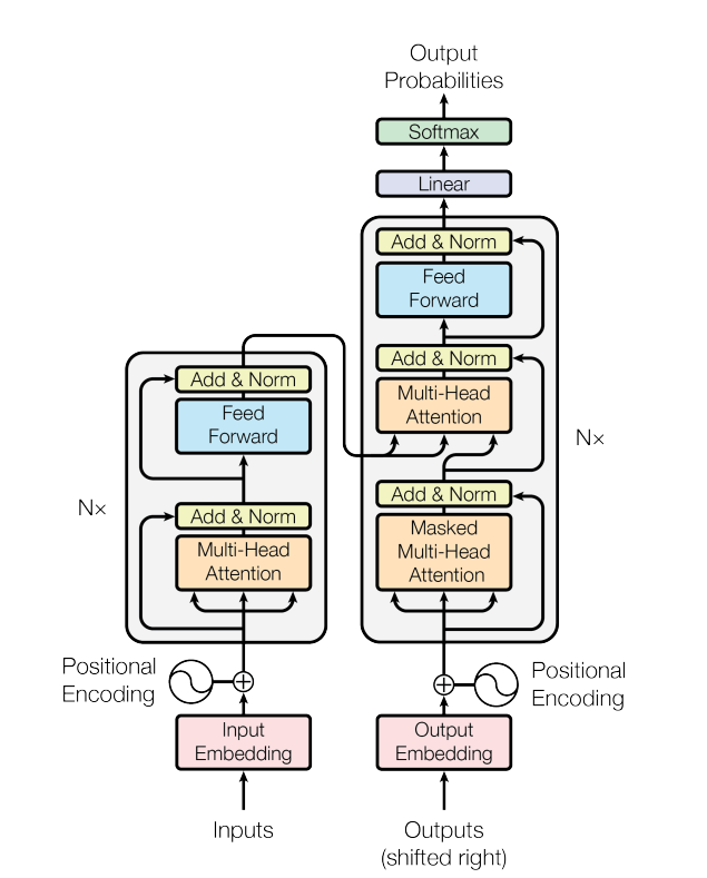
Encoder

Composed of $N=6$ identical layers
Each layer has two sub-layers: Multi-Head Self Attention Mechanism and Point-wise fully connected feed-forward network
Employ a residual connection between two sub-layers, the output of each sub-layer is $LayerNorm(x+Sublayer(x))$

Decoder

Composed of $N=6$ identical layers
in addition to the two sub-layers in encoder, a third sub-layer which performs multi-head attention over the output of the encoder stack is added.
Employ a residual connection between two sub-layers, the output of each sub-layer is $LayerNorm(x+Sublayer(x))$
Modify the self-attention sub-layer to prevent positions from attending to subsequent positions by masks. This can ensure that the predictions for position $i$ can depend only on the known outputs at positions less than $i$.

In the encoder, sequences are consumed to get a feature representation. So the encoder can be used to obtain sequence vectors for classification tasks. While in the decoder, it consumes sequences before position $i$ to predict the word in position $i$, so the decoder can be used to generate new sequences. During training time, if no masks are adopted, self attention mechanism will see the words of the whole sequence and there is no need to predict since we have known the whole sequence.

There are many common components in encoder and decoder: Multi-Head Attention, Position-wise fully connected network, etc. I will discuss about these first then dive into other components in the decoder.

Attention

An attention function can be described as mapping a query and a set of key-valued pairs to an output, where the query, keys, values, and output are all vectors. The output is computed as a weighted sum of the values, where the weight assigned to each value is computed by a compatibility function of the query with the corresponding key.

Intuition behind this attention formulation:

Given a set of vectors $V$, I’d like to get a weighted sum of $V_i$ according to my query $Q$, namely, $\sum_i^n a_i V_i$ , constraint to $\sum_i^n a_i=1$, but how to allocate the weights $a_1, a_2, …, a_n$ properly. Each $V_i$ has $K_i$ , which is used to calculate the relation between $Q$ and $V$. We can get the weights $a$ based on $Q$ and $V$ then get the weighted sum of $V$. In the encoder-decoder architecture, $V=K$, while in self attention mechanism, $Q=K=V$.

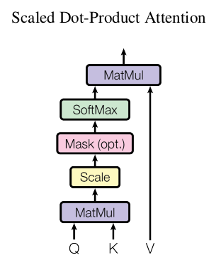
In this paper, the authors proposed scaled dot-product attention, formulated as follows: $Attention(Q,K,V)={\rm softmax} (\frac{QK^T}{\sqrt{d_k}})V$ In this formulation, $\sqrt{d_k}$ is the scaling factor. From the dot expression $QK^T=\sum_i^d Q_i K^T_i$ , we can see that if $d$ is large, the sum value can be very large and it will push the softmax function to regions where it has very small gradients (The authors use the word suspect).

scaled

Multi-Head Attention

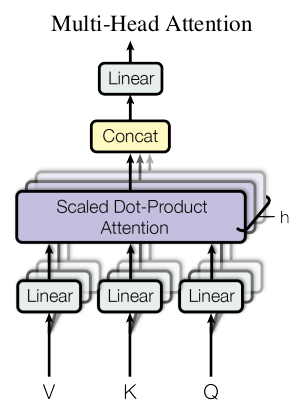
Instead of performing a single attention function with $d_{model}$-dimension keys, values and queries, we found it beneficial to linearly project the queries, keys and values $h$ times with different, learned linear projections to $d_k, d_k$ and $d_v$ dimensions, respectively.

I have read a paper “A Structured Self-attentive Sentence Embedding” which also adopts similar ideas. They both introduce multiple linear projections to the original embeddings.

In this paper, assuming the input dimension is [$B,L,D$] ($B$ is batch size, $L$ is sequence length and $D$ is word vector dimension), for each linear projection $D–>d$ we can get the output [$B,L,d$]. Performing this linear projection $h$ times we can get $h *[B,L,d]$. $d$ can be $d_k$ or $d_v$, $K$ and $V$ are the same and they have the same dimension.

This paper then concatenates the output and once again projects to result in the final values as follows:

$MultiHead(Q,K,V)=Concat(head_1, head_2, ... heawd_h) W^O \\ where head_i=Attention(QW_i^Q, KW_i^K, VW_i^V)$

Dimension:

$W_i^Q \in \mathbb{R}^{d_{model} \times d_k}, W_i^K \in \mathbb{R}^{d_{model} \times d_k}, W_i^V \in \mathbb{R}^{d_{model} \times d_v}$ and $W^O \in \mathbb{R}^{hd_v \times d_{model}}$

$d_{model} $ is the dimension of MultiHead($Q,K,V$) and $d_{model}=h*d_v$.

Project $Q,K,V$ respectively and concatenate the results together, Emmm…Nice!

$QW_i^Q$ projects$ Q$ to $d_k$, $KW_i^k$ projects $K$ to $d_v$, $VW_i^K$ also projects $V$ to $d_v$, then the result dimension should be $d_v$ for each head. $h$ heads should have $h\times d_v$dimension.

Here, $d_k$ and $d_v$ can have different dimensions.

This paper adopts $h=8$ heads, $d_{model}=512$, so $d_k=d_v=d_{model}/h=64$.

Multi-Head

Position-wise Feed-Forward Networks

In the last sub-layer of encoder and decoder, a feed-forward network is applied to perfrom linear transformation as follows: $FFN(x)={\rm max(0,xW_1+b）W_2+b_2}$

The input $x$ is the output of Multi-Head Attention with dimension $d_{model}$. The output dimension is also $d_{model}$. The inner-layer has dimension $d_{ff}=2048$ (Other dimensions are OK).

The authors also put the feed-forward networks in another way:

Another way of describing this is as two convolutions with kernel size 1.

This is the classical problem. How to implement fully-connected network with filters whose kernel size is 1?

Assuming the input dimension is $d_{model}=512$ and the output dimension of the second feed-forward layer is also $d_{model}$. First, we can consider the input as a $1$-d tensor whose depth is $512$, then we can adopt $d_{ff}$ number of $1$ filters with depth $512$. Each filter can get a $1$-dimension result. By performing this $d_{ff}$ times, we can get a $1*d_{ff}$ tensor. Then we can adopt $d_{model}$ of $1$-size filters with depth $d_{ff}$. After performing this $d_{model}$ times, we can get a $1$-d tensor with depth $d_{model}$. So the feed-forward network can also be implemented by two convolutions with kernel size $1$. Conv1d is adopted in PyTorch to implement this function, referring to code below.

Embedding and Softmax

Similarly to other sequence transduction models, we use learned embeddings to convert the input tokens and output tokens to vectors of dimension $d-{model}$. We also use the usual learned linear transformation and softmax function to convert the decoder output to predicted next-token probabilities. In our model, we share the same weight matrix between the two embedding layers and the pre-softmax linear transformations, similar to… In the embedding layers, we multiply those weights by $\sqrt{d_{model}}$.

The Question is “Why do they multiply those weights by $\sqrt{d_{model}}$ ??”

Position Encoding

Since our model contains no recurrence and no convolution, in order for the model to make use of the order of the sequence, we must inject some information about the relative or absolute position of the tokens in the sequence.

The authors adopt relative position to model token sequences as follow:

$PE(pos,2i)=sin(pos/10000^{2i/d_{model}}) \\ PE(pos,2i+1)=cos(pos/10000^{2i/d_{model}})$

where $pos$ is the position and $i$ is the dimension. For each fixed dimension $i$, we can get a sinusoid function. We know that for a sin function: $f(t)=Asin(wt)$, the wavelength(or period $T$) equals $2\pi /w$. For the position function,we can get $T=2\pi / (1/10000^{2i/d_{model}})=2\pi * 10000^{2i/d_{model}}$. We can see that $2i/d_{model}\in [0,1]$. So $T\in [2\pi, 10000 \cdot 2\pi]$. More concisely,

$T \in { 2 \pi, 2 * 2 \pi, 3 * 2 \pi, …, 9999 * 2 \pi, 10000 * 2\pi }$.

Here, $2i$ means even dimensions, and $2i+1$ means odd dimensions, so $i \in {0,1,2,…,d_{model}/2 }$ and $2i/d_{model} \in [0,1]$. Then the functions for each dimension are as follows: sin, cos, sin, cos,…

Then, why relative positions not absolute positions?

We chose this function because we hypothesized it would allow the model to easily to attend by relative positions, since for any fixed offset $k$, $PE_{pos}+k$ can be represented as a linear function of $PE_{pos}$.

Emmm…, it is intuitive and acceptable.

Encoder & Decoder

The encoder represents a sequence as vector representation, and is connected to the downstream tasks. It can replace BiLSTM and be used as a sentence representation method.

The decoder performs similarly to the decoder in seq2seq framework. An encoder contains two sub-layers, and a decoder consists of three sub-layers. Encoder: Multi-Head–> Feed-Forward, Decoder: Multi-Head–>Encoder output–> Feed-Forward. In the decoder, it adopts the outputs of the encoder to calculate the context vector and predict the output word at one step. The the output at step $i$ is fed into the decoder and predicts the next word $i+1$.

So, the encoder can be used as a representation method, while the decoder is similar to the decoder of seq2seq framework.

Why Self Attention?

Three reasons:

The total computation complexity per layer;
The amount of computation that can be parallelized;
The path length between long-range dependencies in the network.

complexity

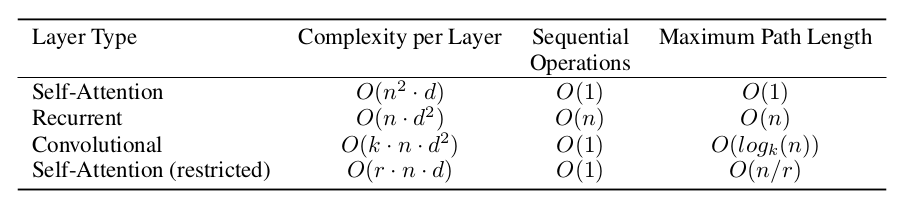
Complexity per Layer

Self-Attention: Dot product, $n$ length, $O(n^2)$ operation, each operation $O(d)$ –> $O(n^2d)$
Recurrent: $n$ length, each step $O(d^2)$ –> $O(nd^2)$
Convolutional: each filter $O(nd^2)$, $k$ filters –> $(knd^2)$
Self-Attention(restricted): similar to self attention, $O(n^2d)$–>$O(rnd)$

Sequential Operation

Recurrent $O(n)$, it needs to consume inputs one by one. The others consumes all the inputs at one time $O(1)$.

Maximum Path Length

This means the maximum path length between two words. In Recurrent, the path length is the absolute position between two words and the maximum is $n$. In self attention, the path is $1$ since each word can interact with other words directly. For self attention (restricted), the width is $n/r$, so the maximum pathh length is $O(n/r)$. For convolutional, $O(log_k(n))$, needs to write more clearly.

As side benefit, self-attention could yield more interpretable models. We inspect attention distributions from our models and present and discuss example. Not only do individual attention heads clearly learn to perform different tasks, many appear to exhibit behavior related to the syntactic and semantic structure of the sentences.

example1

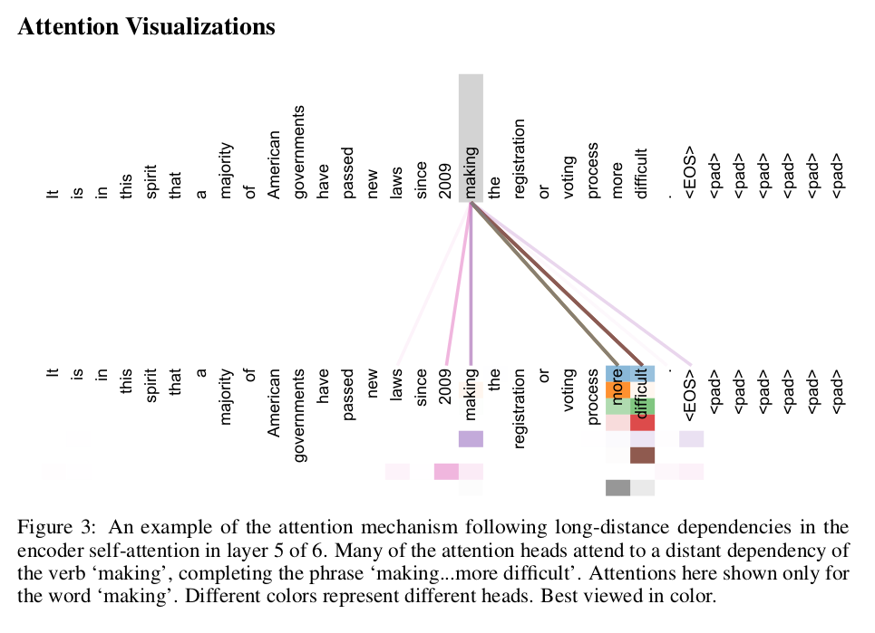
The attention in layer 5 of 6. From the picture, we can see that the word ‘making’ have strong connection with words ‘more’ and ‘difficult’, thus leading to the phrase structure ‘making … more difficult’. Each color means a head attention (totally 8). We can see that many attentions extract the relations between ‘making’ and ‘more’, between ‘making’ and ‘difficult’, so they will have stronger connections.

The problem is, how to generate a picture like this? Assumption: $d=64, h=8, d_{model}=512, d_{model}=d*h$.

In this picture, we should show the attention matrix respectively. For each head, it performs attention on the $d$ vectors, and will generate a $nn$ attention matrix. We should show the $nn$ attention matrix. For each attention, we show it in one color horizontally. The darker the color is, the bigger weight the attention has. When multiple attentions discover the relations between two words, they will have much stronger connections.

example2

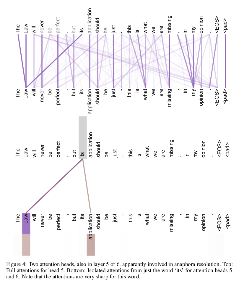
Above: The full attention heads(8) for each word.

Below: Two attention heads(totally 8) for the word ‘its’.

example3

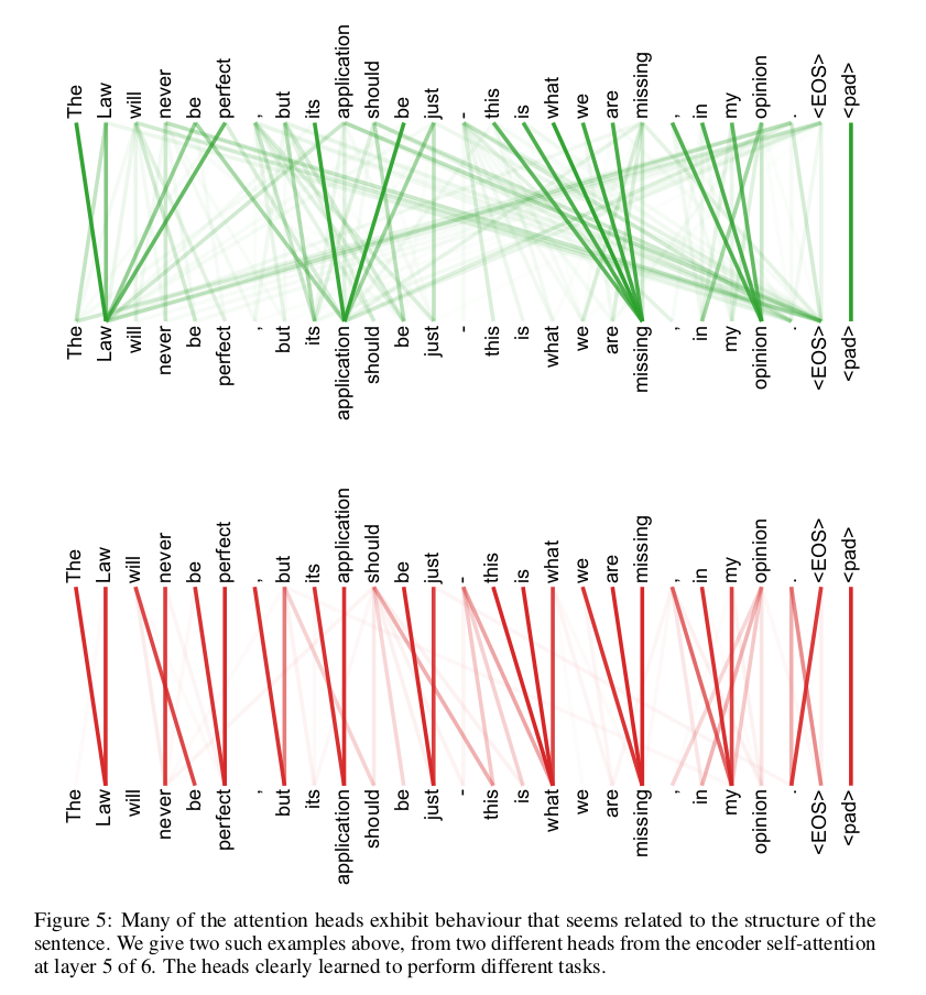
Different attention heads tend to focus on different aspects between sentences. Figure 5 gives two examples of two different heads. The attentions are different, which indicates they focus on diverse aspects we desire. Emmm… The explanation is intuitive and the examples shown are good enough to support this idea. Maybe other attentions are not clear enough.

Experiments

Emmm… I will not write. HHaaaa…

Code release tensorflow: tensor2tensor

Pytorch Implementation

Transformer Pytorch Github

Transformer

class Transformer(nn.Module):
    ''' A sequence to sequence model with attention mechanism. '''

    def __init__(
            self,
            n_src_vocab, n_tgt_vocab, len_max_seq,
            d_word_vec=512, d_model=512, d_inner=2048,
            n_layers=6, n_head=8, d_k=64, d_v=64, dropout=0.1,
            tgt_emb_prj_weight_sharing=True,
            emb_src_tgt_weight_sharing=True):

        super().__init__()

        self.encoder = Encoder(
            n_src_vocab=n_src_vocab, len_max_seq=len_max_seq,
            d_word_vec=d_word_vec, d_model=d_model, d_inner=d_inner,
            n_layers=n_layers, n_head=n_head, d_k=d_k, d_v=d_v,
            dropout=dropout)

        self.decoder = Decoder(
            n_tgt_vocab=n_tgt_vocab, len_max_seq=len_max_seq,
            d_word_vec=d_word_vec, d_model=d_model, d_inner=d_inner,
            n_layers=n_layers, n_head=n_head, d_k=d_k, d_v=d_v,
            dropout=dropout)

        self.tgt_word_prj = nn.Linear(d_model, n_tgt_vocab, bias=False)
        nn.init.xavier_normal_(self.tgt_word_prj.weight)

        assert d_model == d_word_vec, \
        'To facilitate the residual connections, \
         the dimensions of all module outputs shall be the same.'

        if tgt_emb_prj_weight_sharing:
            # Share the weight matrix between target word embedding & the final logit dense layer
            self.tgt_word_prj.weight = self.decoder.tgt_word_emb.weight
            self.x_logit_scale = (d_model ** -0.5)
        else:
            self.x_logit_scale = 1.

        if emb_src_tgt_weight_sharing:
            # Share the weight matrix between source & target word embeddings
            assert n_src_vocab == n_tgt_vocab, \
            "To share word embedding table, the vocabulary size of src/tgt shall be the same."
            self.encoder.src_word_emb.weight = self.decoder.tgt_word_emb.weight

    def forward(self, src_seq, src_pos, tgt_seq, tgt_pos):

        tgt_seq, tgt_pos = tgt_seq[:, :-1], tgt_pos[:, :-1]

        enc_output, *_ = self.encoder(src_seq, src_pos)
        dec_output, *_ = self.decoder(tgt_seq, tgt_pos, src_seq, enc_output)
        seq_logit = self.tgt_word_prj(dec_output) * self.x_logit_scale

        return seq_logit.view(-1, seq_logit.size(2))

The class Transformer is composed of encoders and decoders. In the function forward, first encoder, then encoder, and return the predicted seq_logit. If we perform Transformer on a classification task, then the decoder can be removed and return the output of encoders( The last layer or all the layers).

Encoder

class EncoderLayer(nn.Module):
    ''' Compose with two layers '''

    def __init__(self, d_model, d_inner, n_head, d_k, d_v, dropout=0.1):
        super(EncoderLayer, self).__init__()
        self.slf_attn = MultiHeadAttention(
            n_head, d_model, d_k, d_v, dropout=dropout)
        self.pos_ffn = PositionwiseFeedForward(d_model, d_inner, dropout=dropout)

    def forward(self, enc_input, non_pad_mask=None, slf_attn_mask=None):
        enc_output, enc_slf_attn = self.slf_attn(
            enc_input, enc_input, enc_input, mask=slf_attn_mask)
        enc_output *= non_pad_mask

        enc_output = self.pos_ffn(enc_output)
        enc_output *= non_pad_mask

        return enc_output, enc_slf_attn

The encoder is composed of two parts: MultiHeadAttention and PositionwiseFeedForward. In the forward function, first multi-head, then feed forward and return the output enc_output and self attentions enc_slf_attn. The code is easy to understand.

Decoder

class DecoderLayer(nn.Module):
    ''' Compose with three layers '''

    def __init__(self, d_model, d_inner, n_head, d_k, d_v, dropout=0.1):
        super(DecoderLayer, self).__init__()
        self.slf_attn = MultiHeadAttention(n_head, d_model, d_k, d_v, dropout=dropout)
        self.enc_attn = MultiHeadAttention(n_head, d_model, d_k, d_v, dropout=dropout)
        self.pos_ffn = PositionwiseFeedForward(d_model, d_inner, dropout=dropout)

    def forward(self, dec_input, enc_output, non_pad_mask=None, slf_attn_mask=None, dec_enc_attn_mask=None):
        dec_output, dec_slf_attn = self.slf_attn(
            dec_input, dec_input, dec_input, mask=slf_attn_mask)
        dec_output *= non_pad_mask

        dec_output, dec_enc_attn = self.enc_attn(
            dec_output, enc_output, enc_output, mask=dec_enc_attn_mask)
        dec_output *= non_pad_mask

        dec_output = self.pos_ffn(dec_output)
        dec_output *= non_pad_mask

        return dec_output, dec_slf_attn, dec_enc_attn

The decoder consists of three components: first MultiHeadAttention , second the output of encoder self.enc_attn which is also a MultiHeadAttentionf function, then PositionwiseFeedForward. During the running time, first slf_attn and enc_attn with mask, next pos_ffn. It follows the process in the paper and is easy to understand. Finally, return dec_output, dec_slf_attn and dec_enc_attn for different purposes.

Multi-Head Attention

class MultiHeadAttention(nn.Module):
    ''' Multi-Head Attention module '''

    def __init__(self, n_head, d_model, d_k, d_v, dropout=0.1):
        super().__init__()

        self.n_head = n_head
        self.d_k = d_k
        self.d_v = d_v 

        self.w_qs = nn.Linear(d_model, n_head * d_k)
        self.w_ks = nn.Linear(d_model, n_head * d_k)
        self.w_vs = nn.Linear(d_model, n_head * d_v)
        nn.init.normal_(self.w_qs.weight, mean=0, std=np.sqrt(2.0 / (d_model + d_k)))
        nn.init.normal_(self.w_ks.weight, mean=0, std=np.sqrt(2.0 / (d_model + d_k)))
        nn.init.normal_(self.w_vs.weight, mean=0, std=np.sqrt(2.0 / (d_model + d_v)))

        self.attention = ScaledDotProductAttention(temperature=np.power(d_k, 0.5))
        self.layer_norm = nn.LayerNorm(d_model)

        self.fc = nn.Linear(n_head * d_v, d_model)
        nn.init.xavier_normal_(self.fc.weight)

        self.dropout = nn.Dropout(dropout)


    def forward(self, q, k, v, mask=None):
 
        d_k, d_v, n_head = self.d_k, self.d_v, self.n_head

        sz_b, len_q, _ = q.size()
        sz_b, len_k, _ = k.size()
        sz_b, len_v, _ = v.size()

        residual = q

        q = self.w_qs(q).view(sz_b, len_q, n_head, d_k)
        k = self.w_ks(k).view(sz_b, len_k, n_head, d_k)
        v = self.w_vs(v).view(sz_b, len_v, n_head, d_v)

        q = q.permute(2, 0, 1, 3).contiguous().view(-1, len_q, d_k) # (n*b) x lq x dk
        k = k.permute(2, 0, 1, 3).contiguous().view(-1, len_k, d_k) # (n*b) x lk x dk
        v = v.permute(2, 0, 1, 3).contiguous().view(-1, len_v, d_v) # (n*b) x lv x dv

        mask = mask.repeat(n_head, 1, 1) # (n*b) x .. x ..
        output, attn = self.attention(q, k, v, mask=mask)

        output = output.view(n_head, sz_b, len_q, d_v)
        output = output.permute(1, 2, 0, 3).contiguous().view(sz_b, len_q, -1) # b x lq x (n*dv)

        output = self.dropout(self.fc(output))
        output = self.layer_norm(output + residual)

        return output, attn

MultiHeadAttention is a basic components of both encoder and decoder and is the key component of Transformer. I will write it in details.

In this paper, n_head=8, d_model=512, d_k=d_v=64.

self.w_qs = nn.Linear(d_model, n_head * d_k)
self.w_ks = nn.Linear(d_model, n_head * d_k)
self.w_vs = nn.Linear(d_model, n_head * d_v)

self.w_qs, self.w_ks and self.w_vs correspond to $W_i^Q, W_i^K, W_i^V \in \mathbb{R}^{d_{model}\times d_k}$ , respectively. d_model equals d_word_vec for calculation convenience. If d_model=512 then word vector dimension should be 512… But we can also add a linear transformation [d_word_vec, d_model] and the constraint can be relaxed.

q = self.w_qs(q).view(sz_b, len_q, n_head, d_k)
k = self.w_ks(k).view(sz_b, len_k, n_head, d_k)
v = self.w_vs(v).view(sz_b, len_v, n_head, d_v)

After performing self.w_qs(q), q is [sz_b,len_q, n_head*d_k]. Then a view operation changes the dimension to [sz_b, len_q, n_head, d_k].

q = q.permute(2, 0, 1, 3).contiguous().view(-1, len_q, d_k) # (n*b) x lq x dk
k = k.permute(2, 0, 1, 3).contiguous().view(-1, len_k, d_k) # (n*b) x lk x dk
v = v.permute(2, 0, 1, 3).contiguous().view(-1, len_v, d_v) # (n*b) x lv x dv

This operation permutes q to [sz_b*n_head,len_q,d_k ]. Err…. for self attention. sz_b*n_headnumbers of self attention which performs on [leq_d, d_k] and it gets a[sz_b*n_head,leq_d, leq_d] attention tensor.

After self attention, resize the output:

output = output.view(n_head, sz_b, len_q, d_v)
output = output.permute(1, 2, 0, 3).contiguous().view(sz_b, len_q, -1) # b x lq x (n*dv)

Then return the results: attn and output.

temperature: the scaled factor $\sqrt{d}$ .

Point-Wise Feed Forward

class PositionwiseFeedForward(nn.Module):
    ''' A two-feed-forward-layer module '''

    def __init__(self, d_in, d_hid, dropout=0.1):
        super().__init__()
        self.w_1 = nn.Conv1d(d_in, d_hid, 1) # position-wise
        self.w_2 = nn.Conv1d(d_hid, d_in, 1) # position-wise
        self.layer_norm = nn.LayerNorm(d_in)
        self.dropout = nn.Dropout(dropout)

    def forward(self, x):
        residual = x
        output = x.transpose(1, 2)
        output = self.w_2(F.relu(self.w_1(output)))
        output = output.transpose(1, 2)
        output = self.dropout(output)
        output = self.layer_norm(output + residual)
        return output

Emmm… This implements by convolution operations, not feed-forward network.

self.w_1 = nn.Conv1d(d_in, d_hid, 1) # position-wise
self.w_2 = nn.Conv1d(d_hid, d_in, 1) # position-wise

For nn.Conv1d:

Args:
    in_channels (int): Number of channels in the input image
    out_channels (int): Number of channels produced by the convolution
    kernel_size (int or tuple): Size of the convolving kernel

For a vector with dimension k, we can regard it as a 1 vector whose depth k. Then the input channel is d_in. If we adopt d_out filters, the output dimension will be d_out. In my opinion, nn.Conv1d is the same with nn.Linear. The number of parameters is d_in * d_out.

After dropout and layer_norm, return output. The output will be the input of the next Encoder block. So the dimension of output should be d_model. (For the first encoder block: d_model=d_word_vec).

Scaled Dot Product Attention

class ScaledDotProductAttention(nn.Module):
    ''' Scaled Dot-Product Attention '''

    def __init__(self, temperature, attn_dropout=0.1):
        super().__init__()
        self.temperature = temperature
        self.dropout = nn.Dropout(attn_dropout)
        self.softmax = nn.Softmax(dim=2)

    def forward(self, q, k, v, mask=None):

        attn = torch.bmm(q, k.transpose(1, 2))
        attn = attn / self.temperature

        if mask is not None:
            attn = attn.masked_fill(mask, -np.inf)

        attn = self.softmax(attn)
        attn = self.dropout(attn)
        output = torch.bmm(attn, v)

        return output, attn

$Attention(Q,K,V)={\rm softmax}(\frac{QK^T}{\sqrt{d_k}})V$

Position Embedding

def get_sinusoid_encoding_table(n_position, d_hid, padding_idx=None):
    ''' Sinusoid position encoding table '''

    def cal_angle(position, hid_idx):
        return position / np.power(10000, 2 * (hid_idx // 2) / d_hid)

    def get_posi_angle_vec(position):
        return [cal_angle(position, hid_j) for hid_j in range(d_hid)]

    sinusoid_table = np.array([get_posi_angle_vec(pos_i) for pos_i in range(n_position)])

    sinusoid_table[:, 0::2] = np.sin(sinusoid_table[:, 0::2])  # dim 2i
    sinusoid_table[:, 1::2] = np.cos(sinusoid_table[:, 1::2])  # dim 2i+1

    if padding_idx is not None:
        # zero vector for padding dimension
        sinusoid_table[padding_idx] = 0.

    return torch.FloatTensor(sinusoid_table)

Position Embedding has been illustrated in details above.

$PE(pos,2i)=sin(pos/10000^{2i/d_{model}}) \\ PE(pos,2i+1)=cos(pos/10000^{2i/d_{model}})$

Conclusion

Transformer is composed of encoders and decoders. Each encoder contains two components: Multi-Head Attention and Point-Wise Feed Forward. Each decoder contains three components: Multi-Head Attention, encoder output, Point-Wise Feed Forward.
The encoder can replace BiLSTM for sequence modeling in NLI, MRC or other classification taks, etc. The decoder can be used on generation problems.
Transformer can relieve the long-dependency problems and can be implemented in parallelism.
For Multi-Head Attention, please add some attention heat-maps in your paper. The reviewers are pleased to see pictures ^-^.